Word Embeddings in Natural Language Processing(NLP)

The article contains insights into the techniques for creating the numerical representation of the data so that it can be acted on by mathematical and statistical models.

Image Credits

Introduction

In natural language processing (NLP), word embedding is a term used for the representation of words for text analysis, typically in the form of a real-valued vector that encodes the meaning of the word such that the words that are closer in the vector space are expected to be similar in meaning.

Why do we need Word Embeddings?

As we know the machine learning models cannot process text so we need to figure out a way to convert these textual data into numerical data. Previously techniques like Bag of Words, Count Vectorizer, and TF-IDF have been discussed that can help achieve use this task. Apart from this, we can use two more techniques such as one-hot encoding, or we can use unique numbers to represent words in a vocabulary. The latter approach is more efficient than one-hot encoding as instead of a sparse vector, we now have a dense one. Thus this approach even works when our vocabulary is large.

In the below example, Imagine if you had 3 categories of foods: apples, chicken, and broccoli. Using label encoding, you would assign each of these an integer number to categorize them: Apple = 1, Chicken = 2, and Broccoli = 3. But now, if your model internally needs to calculate the average across categories, it might do 1+3 = 4/2 = 2. This means that according to your model, the average of apples and chicken together is broccoli.

Obviously, that line of thinking by your model is going to lead to it getting correlations completely wrong, that is the reason one-hot encoding is preferred over label encoding.

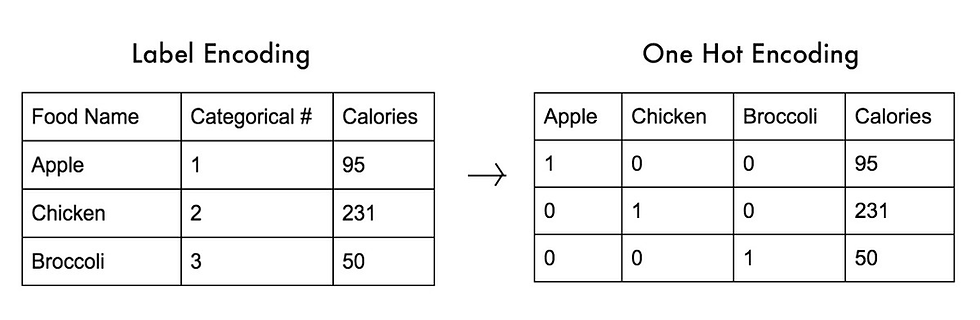
Label encoding vs One-hot encoding. Credits

However, Neither One-hot encoding nor Label encoding captures any relationship between these words. It can be challenging for a model to interpret, for example, a linear classifier learns a single weight for each feature. Because there is no relationship between the similarity of any two words and the similarity of their encodings, this feature-weight combination is not meaningful.

Secondly, One-hot encoding will create high dimensional sparse matrices for each word then obviously it will be very difficult to get the similarity between words and get the sematic information about these words.

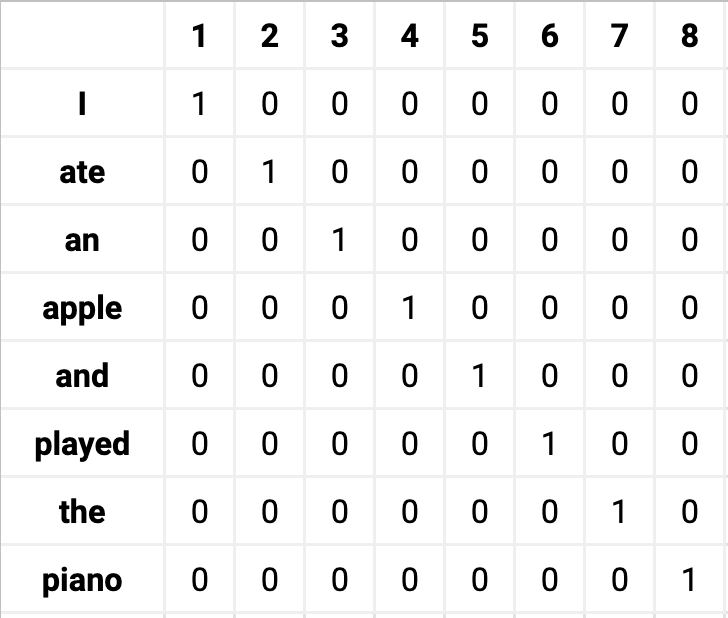
High dimensional sparse matrix generated by One-Hot encoding. Credits

Thus by using word embeddings, words that are close in meaning are grouped near to one another in vector space. For example, while representing a word such as frog, the nearest neighbor of a frog would be frogs, toads, Litoria. This implies that it is alright for a classifier to not see the word Litoria and only frog during training, and the classifier would not be thrown off when it sees Litoria during testing because the two-word vectors are similar. Also, word embeddings learn relationships. Vector differences between a pair of words can be added to another word vector to find the analogous word.

For example, “man” -“woman” + “queen” ≈ “king”.

What is Word Embeddings?

Word embeddings are a type of word representation that allows words with similar meanings to have a similar representation. They are a distributed representation for the text that is perhaps one of the key breakthroughs for the impressive performance of deep learning methods on challenging natural language processing problems.

Word embeddings are in fact a class of techniques where individual words are represented as real-valued vectors in a predefined vector space. Each word is mapped to one vector and the vector values are learned in a way that resembles a neural network, and hence the technique is often lumped into the field of deep learning. The distributed representation is learned based on the usage of words. This allows words that are used in similar ways to result in having similar representations, naturally capturing their meaning.

Neural network embeddings have 3 primary purposes:

• Finding nearest neighbors in the embedding space. These can be used to make recommendations based on user interests or cluster categories.

• As input to a machine learning model for a supervised task.

• For visualization of concepts and relations between categories.

Word2Vec

One of the most popular algorithms in the word embedding space has been Word2Vec. It was the first widely disseminated word embedding method and was developed by Tomas Mikolov, a researcher at Google.

Word2Vec converts words in a vector space representation. This vector representation is done such that similar words are placed close to each other while dissimilar words are way far apart. Technically, word2vec uses the semantic relationship between words for vector representation.

Also, word2vec checks for the linguistics context of words in a sentence. By context, we mean words that surround a particular word in a sentence. When communicating as humans, we use context to understand what the other party is saying.

If for instance, you read the statement “The man was dozing at work”. You may quickly conclude that he must be a lazy man to be dozing at work. But if only some context was added. Let’s say it now reads this way. “The man stayed up all night to finish his presentation slide. When he got to work the following morning, he was dozing at work”. The extra content provided the context that completely changes our perspective about the man. Now you won’t see him as a lazy man but as a human who needs some rest. That’s how powerful context is.

Architecture

Word2Vec offers two neural network-based variants:

1. Continuous Skip-gram model

2. Continuous-Bag-Of-Words model (CBOW).

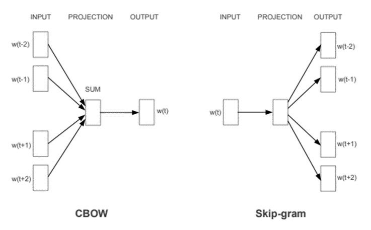
CBOW & Skip-gram architectures.The CBOW architecture predicts the current word based on the context, and the Skip-gram predicts surrounding words given the current word. . Credits: Word2Vec paper

Continuous bag of words(CBOW) models learn word embedding by predicting the present word based on the context of the corpus. The continuous skip-gram model, on the other hand, learns by predicting the surrounding based solely on the present word.

CBOW is quite faster than continuous skip-gram and represents common words better in the text whereas skip-gram needs an amount of data and is good at representing uncommon words or phrases in the data.

CBOW is quick and finds better numerical representations for frequent words, while Skip Gram can efficiently represent rare words. Word2Vec models are good at capturing semantic relationships among words. For example, the relationship between a country and its capital, like Paris is the capital of France and Berlin is the capital of Germany. It is best suited for performing semantic analysis, which has application in recommendation systems and knowledge discovery.

In both methods, however, the learning takes paces based on the usage of surrounding words. This method provides better word embedding learning with low space and lesser computational time. This allows for embeddings from large texts, and that is to the tune of billions of words.

GloVe (Global Vectors for Word Representation)

GloVe extends the work of Word2Vec to capture global contextual information in a text corpus by calculating a global word-word co-occurrence matrix.

Word2Vec only captures the local context of words. During training, it only considers neighboring words to capture the context. GloVe considers the entire corpus and creates a large matrix that can capture the co-occurrence of words within the corpus.

GloVe mixes the advantages of two-word vector learning methods: matrix factorization like latent semantic analysis (LSA) and local context window method like Skip-gram. The GloVe technique has a simpler least square cost or error function that reduces the computational cost of training the model. The resulting word embeddings are different and improved.

GloVe performs significantly better in word analogy and named entity recognition problems. It is better than Word2Vec in some tasks and competes in others. However, both techniques are good at capturing semantic information within a corpus.

FastText

FastText is another word embedding method that is an extension of the word2vec model. Instead of learning vectors for words directly, FastText represents each word as an n-gram of characters. So, for example, take the word, “artificial” with n=3, the fastText representation of this word is <ar, art, rti, tif, ifi, fic, ici, ial, al>, where the angular brackets indicate the beginning and end of the word.

This helps capture the meaning of shorter words and allows the embeddings to understand suffixes and prefixes. Once the word has been represented using character n-grams, a skip-gram model is trained to learn the embeddings. This model is considered to be a bag of words model with a sliding window over a word because no internal structure of the word is taken into account. As long as the characters are within this window, the order of the n-grams doesn’t matter.

If we denote n-gram vector as z and v as an output vector representation of word w (context word):

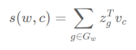
We can choose n-grams of any size, but in practice size from 3 to 6 is the most suitable one.

FastText works well with infrequent words. So even if a word wasn’t seen during training, it can be broken down into n-grams to get its embeddings.

Word2vec and GloVe both fail to provide any vector representation for words that are not in the model dictionary. This is a huge advantage of this method.

BERT(Bidirectional Encoder Representations from Transformers)

For generating word embeddings, BERT relies on an attention mechanism. It generates high-quality context-aware or contextualized word embeddings. During the training process, embeddings are distilled by passing through each BERT encoder layer. For each word, the attention mechanism captures word associations based on the words on the left and the words on the right. Word embeddings are also positionally encoded to keep track of the pattern or position of each word in a sentence.

BERT is more advanced than any of the techniques discussed above. It creates more reasonable word embeddings as the model is pre-trained on enormous word corpus and Wikipedia datasets. BERT can be enhanced by fine-tuning the embeddings on task-specific datasets.

Though, BERT is most fit for language translation tasks. It has been optimized for many other applications and domains.

Implementing pre-trained word embedding: GloVe

We will use the glove.6B.100d.txt file containing the glove vectors trained on the Wikipedia and GigaWord datasets.

Load the libraries:

import pandas as pd
import numpy as np
import os
import matplotlib.pyplot as plt
import seaborn as sn
import pickle

%matplotlib inline

#Import module to split the datasets
from sklearn.model_selection import train_test_split
# Import modules to evaluate the metrics
from sklearn import metrics
from sklearn.metrics import confusion_matrix,accuracy_score,roc_auc_score,roc_curve,auc

We set the variables for data location.

# Global parameters
#root folder
root_folder='.'
data_folder_name='data'
glove_filename='/content/drive/MyDrive/glove.6B.100d.txt'

train_filename='train.csv'
# Variable for data directory
DATA_PATH = os.path.abspath(os.path.join(root_folder, data_folder_name))
glove_path = os.path.abspath(os.path.join(DATA_PATH, glove_filename))

# Both train and test set are in the root data directory
train_path = DATA_PATH
test_path = DATA_PATH

#Relevant columns
TEXT_COLUMN = 'text'
TARGET_COLUMN = 'target'

First, we convert the GloVe file containing the word embeddings to the word2vec format for the convenience of use.

from gensim.scripts.glove2word2vec import glove2word2vec

word2vec_output_file = glove_filename+'.word2vec'
glove2word2vec(glove_path, word2vec_output_file)

So our vocabulary contains 400K words represented by a feature vector of shape 100. Now we can load the Glove embeddings in word2vec format and then analyze some analogies. In this way, if we want to use pre-trained word2vec embeddings we can simply change the filename and reuse all the code below.

from gensim.models import KeyedVectors
# load the Stanford GloVe model
word2vec_output_file = glove_filename+'.word2vec'
model = KeyedVectors.load_word2vec_format(word2vec_output_file, binary=False)

#Show a word embedding
print('King: ',model.get_vector('king'))

result = model.most_similar(positive=['woman', 'king'], negative=['man'], topn=1)

print('Most similar word to King + Woman: ', result)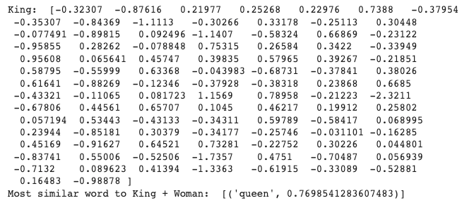

Analyzing the vector space and finding analogies

We would like to extract some interesting features of our word embeddings, Now, our words are numerical vectors so we can measure and compare distances between words to show some of the properties that these embedding provide.

For example, we can compare some analogies. The most famous is the following: king – man + woman = queen. In other words, adding the vectors associated with the words king and woman while subtracting man is equal to the vector associated with queen. In other words, by subtracting the concept of man from the concept of King we get a representation of the "royalty". Then, if we sum to the woman word this concept we obtain the word "queen". Another example is France – Paris + Rome = Italy. In this case, the vector difference between Paris and France captures the concept of a country.

Now we will show some of these analogies on different topics.

result = model.most_similar(positive=['woman', 'king'], negative=['man'], topn=1)
print('King - Man + Woman = ',result)
result = model.most_similar(positive=['rome', 'france'], negative=['paris'], topn=1)
print('France - Paris + Rome = ',result)
result = model.most_similar(positive=['english', 'france'], negative=['french'], topn=1)
print('France - french + english = ',result)
result = model.most_similar(positive=['june', 'december'], negative=['november'], topn=1)
print('December - November + June = ',result)
result = model.most_similar(positive=['sister', 'man'], negative=['woman'], topn=1)
print('Man - Woman + Sister = ',result)

We can observe how the word vectors include information to relate countries with nationalities, months of the year, family relationships, etc.

But not always we get the expected results:

result = model.most_similar(positive=['aunt', 'nephew'], negative=['niece'], topn=1)
print('France - Paris + Rome = ',result)

France - Paris + Rome = [('uncle', 0.8936851024627686)]

We can extract which words are more similar to another word, so they all are "very close" in the vector space.

result = model.most_similar(positive=['india'], topn=10)
print('10 most similar words to India: ',result)

result = model.most_similar(positive=['cricket'], topn=10)
print('\n10 most similar words to Cricket: ',result)

result = model.most_similar(positive=['engineer'], topn=10)
print('\n10 most similar words to Engineer: ',result)

10 most similar words to India: [('pakistan', 0.8370324373245239), ('indian', 0.780203104019165), ('delhi', 0.7712194919586182), ('bangladesh', 0.7661640644073486), ('lanka', 0.7639288306236267), ('sri', 0.7506585121154785), ('australia', 0.7042096853256226), ('malaysia', 0.6796302795410156), ('nepal', 0.6761943697929382), ('thailand', 0.6671633720397949)]

10 most similar words to Cricket: [('rugby', 0.7827098369598389), ('twenty20', 0.7362942695617676), ('england', 0.7173773646354675), ('indies', 0.7157819271087646), ('cricketers', 0.7132172584533691), ('football', 0.6659637093544006), ('zealand', 0.6606223583221436), ('matches', 0.6509107351303101), ('bowling', 0.6504763960838318), ('wc2003-wis', 0.6422653198242188)]

10 most similar words to Engineer: [('engineers', 0.7049852013587952), ('technician', 0.7031464576721191), ('mechanic', 0.669628381729126), ('engineering', 0.6665581464767456), ('architect', 0.6495680809020996), ('contractor', 0.6494842767715454), ('officer', 0.6446554660797119), ('worked', 0.6210095882415771), ('master', 0.616294264793396), ('chemist', 0.6130304336547852)]

result = model.similar_by_word("dog")
print(" Dog is similar to {}: {:.4f}".format(*result[0]))
result = model.similar_by_word("brother")
print(" Brother is similar to {}: {:.4f}".format(*result[0]))

Dog is similar to cat: 0.8798

Brother is similar to son: 0.9376 The idea behind all of the word embeddings is to capture with them as much of the semantical/morphological/context/hierarchical/etc. information as possible, but in practice one methods are definitely better than the other for a particular task (for instance, LSA is quite effective when working in low-dimensional space for the analysis of incoming documents from the same domain zone as the ones, which are already processed and put into the term-document matrix). The problem of choosing the best embeddings for a particular project is always the problem of the try-and-fail approach, so realizing why in a particular case one model works better than the other sufficiently helps in real work.

Visualization of word embeddings

Another exciting operation we can do with embeddings is visualization, plotting them in a 2D dimensional space can show us how words are related. Most similar words should be plotted in groups while non-related words will appear at a large distance. This requires a further dimension reduction technique to get the dimensions to 2 or 3. The most popular technique for reduction is itself an embedding method: t-Distributed Stochastic Neighbor Embedding (TSNE).

t-SNE stands for t-distributed stochastic neighbor embedding. It is a technique for dimensionality reduction that is best suited for the visualization of a high-dimensional dataset.

from sklearn.decomposition import IncrementalPCA    # inital reduction
from sklearn.manifold import TSNE                   # final reduction
import numpy as np                                  # array handling

def display_closestwords_tsnescatterplot(model, dim, words):
    
    arr = np.empty((0,dim), dtype='f')
    word_labels = words

    # get close words
    #close_words = [model.similar_by_word(word) for word in words]
    
    # add the vector for each of the closest words to the array
    close_words=[]
    for word in words:
        arr = np.append(arr, np.array([model[word]]), axis=0)
        close_words +=model.similar_by_word(word)
        
    for wrd_score in close_words:
        wrd_vector = model[wrd_score[0]]
        word_labels.append(wrd_score[0])
        arr = np.append(arr, np.array([wrd_vector]), axis=0)
        
    # find tsne coords for 2 dimensions
    tsne = TSNE(n_components=2, random_state=0)
    #np.set_printoptions(suppress=True)
    Y = tsne.fit_transform(arr)

    x_coords = Y[:, 0]
    y_coords = Y[:, 1]
    # display scatter plot
    plt.scatter(x_coords, y_coords)

    for label, x, y in zip(word_labels, x_coords, y_coords):
        plt.annotate(label, xy=(x, y), xytext=(0, 0), textcoords='offset points')
    plt.xlim(x_coords.min()+0.00005, x_coords.max()+0.00005)
    plt.ylim(y_coords.min()+0.00005, y_coords.max()+0.00005)
    plt.show()
    
def tsne_plot(model, words):
    "Creates and TSNE model and plots it"
    labels = []
    tokens = []

    #for word in model.wv.vocab:
    for word in words:
        tokens.append(model[word])
        labels.append(word)
    
    tsne_model = TSNE(perplexity=40, n_components=2, init='pca', n_iter=2500, random_state=23)
    new_values = tsne_model.fit_transform(tokens)

    x = []
    y = []
    for value in new_values:
        x.append(value[0])
        y.append(value[1])
        
    plt.figure(figsize=(14, 10)) 
    for i in range(len(x)):
        plt.scatter(x[i],y[i])
        plt.annotate(labels[i],
                     xy=(x[i], y[i]),
                     xytext=(5, 2),
                     textcoords='offset points',
                     ha='right',
                     va='bottom')
    plt.show()

For example, we will plot a hundred words from our word embeddings and also the most similar words to the concept of woman and car. All similar words should be plotted closely, while the rest of the words will appear distributed across the vector space:

words=list(model.vocab.keys())
word1 = words[800:870]
words2= model.similar_by_word('woman')
words3= model.similar_by_word('car')
words= word1 + [w[0] for w in words2] + [w[0] for w in words3]
#print(words)
tsne_plot(model, words)

References

https://edumunozsala.github.io/BlogEms/jupyter/nlp/classification/embeddings/python/2020/08/15/Intro_NLP_WordEmbeddings_Classification.html#Loading-a-pre-trained-word-embedding:-GloVe

https://www.mygreatlearning.com/blog/word-embedding/

https://en.wikipedia.org/wiki/Word_embedding

https://www.kdnuggets.com/2021/11/guide-word-embedding-techniques-nlp.html

https://blogs.sap.com/2019/07/03/glove-and-fasttext-two-popular-word-vector-models-in-nlp/